AI-Based Prospective Slice Tracking for Continuous Visualization of Gadolinium-Filled Balloon Wedge Catheters in MRI-Guided Cardiac Catheterization

For the training of robust and reliable convolutional neural networks (CNN) in CMR, the learning environment (LE), including data pre-processing and choice of CNN parameters, plays a crucial role (1,2). In CMR, domain shifts such as different technical setups, sites and patient characteristics, may interfere with CNN performance. Typically, LEs are manually designed by data scientists who finetune them with heuristics and experiments (3,4). Data augmentations increase the performance and generalizability of CNNs across domains by increasing image variability (Fig.1). Optimizing LEs requires determining high-dimensional combinations of many augmentations, their probabilities, and CNN parameters for the training process (5). Typically, LEs are fixed for the entire training process. However, in principle optimal LEs may vary over the training process, called shifting LEs, with different combinations being optimal at different time points.

The aim is to design an evolutionary algorithm that computes shifting LEs for CNNs that predict myocardial segmentations and reference points for parametric mapping.

Methods:

An evolutionary algorithm was designed to train 24 CNNs in parallel to learn contours and reference points. Each CNN is initialized with a random LE. After each train step the CNNs are evaluated on a validation set. The 5 worst performers are replaced with copies of the 5 top performers, then the LE parameters of all CNNs are slightly mutated to explore new combinations (Fig.2). The overall dataset consists of 721 images from 283 patients annotated by a CMR expert with reference points and myocardial contours. Training data was the first half, validation and test data the two last quarters respectively. LE parameter averages were calculated as they evolved. The segmentation performance was evaluated using the Dice similarity coefficient (Dice), the reference point estimation via CNN and expert distance, and overall performance as T1 mean deviations.

Results:

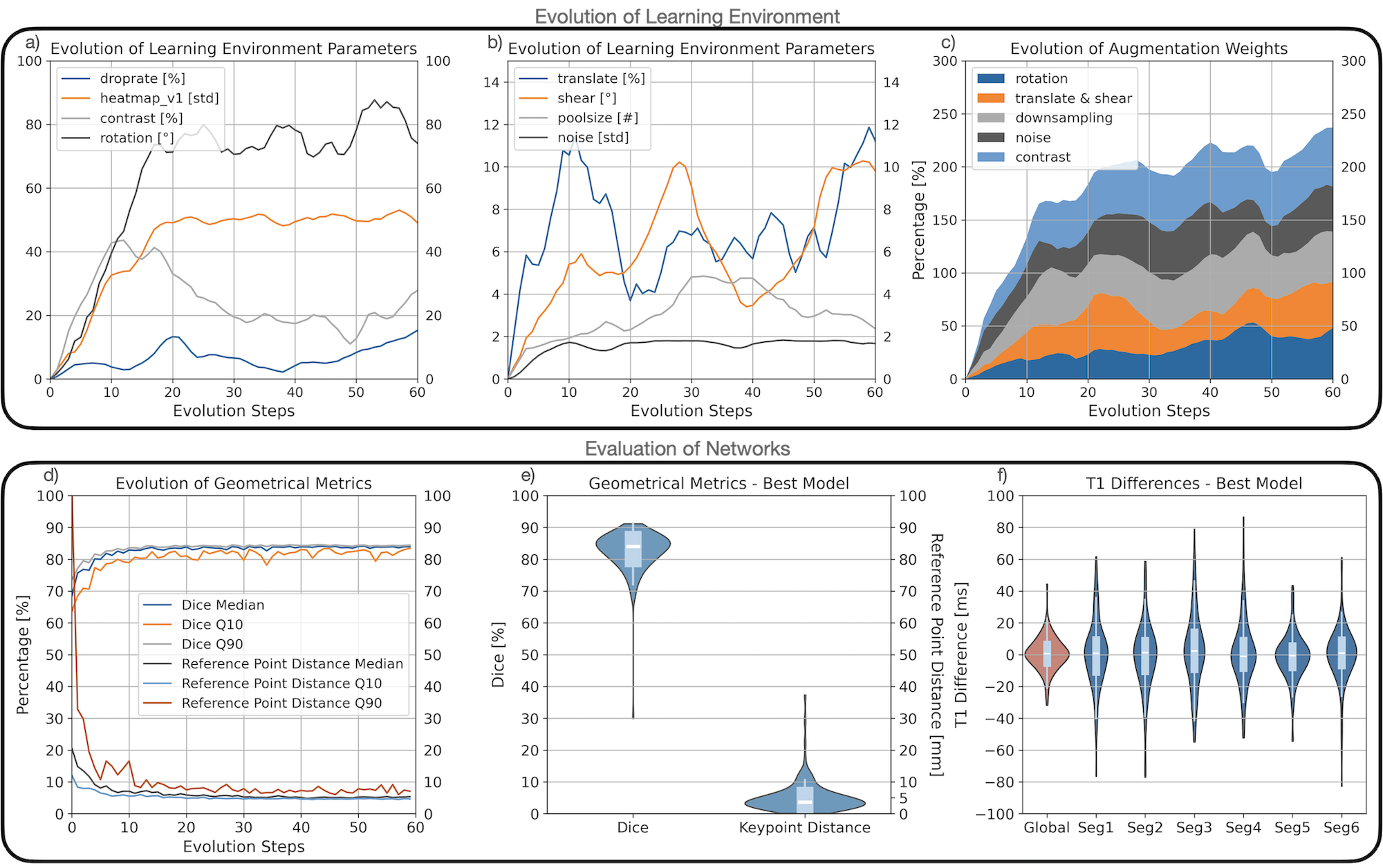
All LE parameters evolved over time with average data augmentation probabilities increasing from 0% to approximately 45% (Fig.3c). The data augmentation parameters for individual operations partially shifted over time (e.g. contrast increased to 45% by train step 10, then decreased to 18% by train step 40), others remained stationary after an initial increase (e.g. rotation plateaued after 20 train steps) (Fig.3a). Average CNN performances improved during evolution: Dice increased to 84%, and reference point distance decreased to 5mm (Fig.3d). The best performing CNN was evaluated on an unseen test dataset. Its performance was Dice: 84%, reference point distance: 5mm (Fig.3e), T1 global difference: -1ms, and segmental differences between -2 and 0 (Fig.3f).

Conclusion:

The evolutionary algorithm optimizes shifting learning environments effectively, producing high-performing CNNs for T1 image segmentation and reference point estimation. The generic approach should generalize well to other optimization problems.

Figure 1: Learning Environments for Robust Neural Networks Learning Environments (LE) describe a set of parameters often associated with convolutional neural network training. LEs encompass data augmentations (a), output adaptions (b), and architectural parameters (c). Data augmentations (a) are image transformations that alter original images with challenging distortions (e.g. downsampling of images or increasing their contrast); this results in a larger and artificially enhanced training dataset. Outputs of CNNs (c) are typically arbitrary feature maps, for example segmentation masks from which contours are extracted, or heatmaps from which reference points are calculated. The variance of the Gaussian heatmaps may be altered in order to improve the training performance. An architectural parameters that may affect the robustness (c) is the dropout rate, which forces the CNN to remain stable when individual neurons are deactivated (removed neurons in red).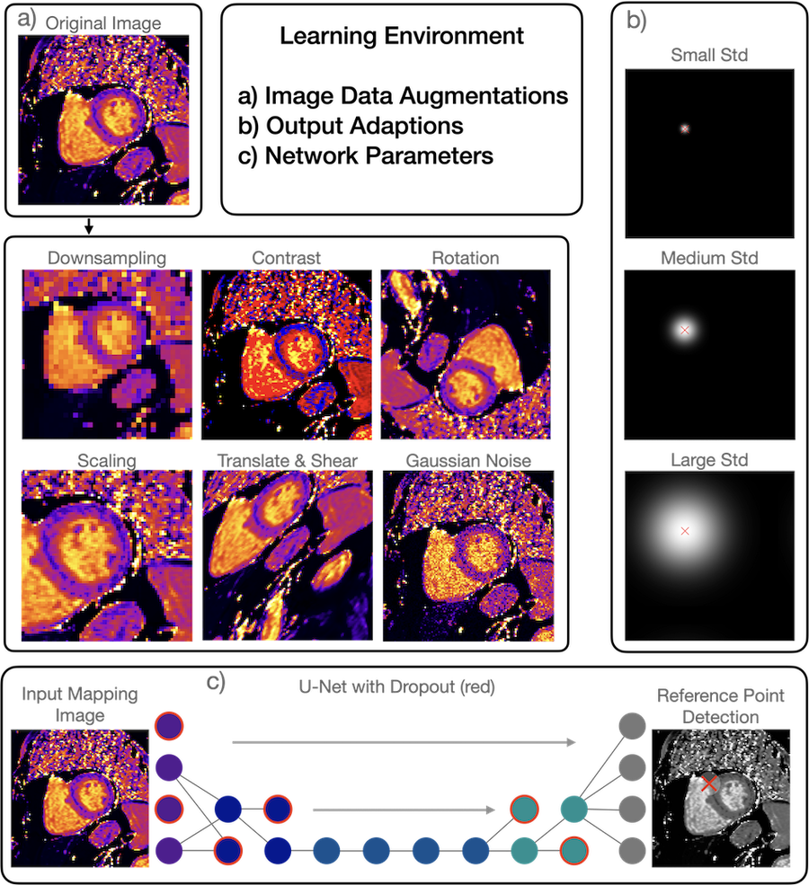

Figure 2: Evolutionary Algorithm for Shifting Learning Environments A population of CNNs is initialized with randomly selected learning environment parameters. Parameters include CNN hyperparameters (cogwheel icons) and data augmentation parameters (book icons). The CNNs are trained iteratively and then evaluated on a validation dataset. CNN members are selected for high performance on the validation data. High performers replace poor performers (e.g. the first CNN LE is replaced with the blue one’s), then all LEs are mutated (i.e. their parameters are slightly altered). Finally, the best CNN is selected as the algorithm’s output.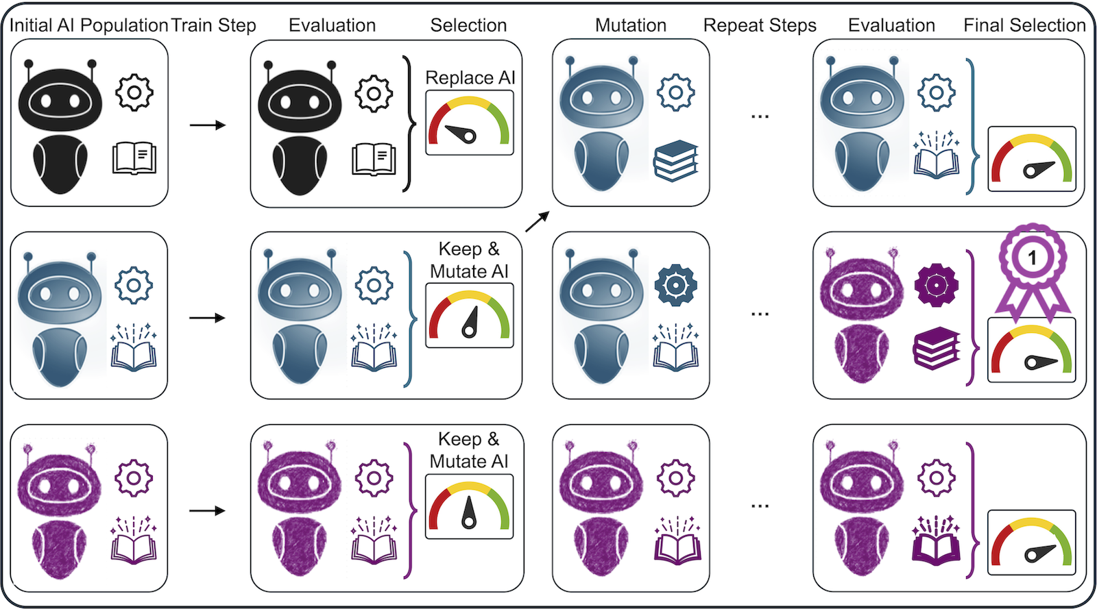

Figure 3: Evaluation of Learning Environments and Neural Network Performances The upper subfigures (a,b,c) show the evolution of the learning environments as average values. In a) and b) the evolution of the augmentation specific parameters is presented, such as the maximal angle for the rotation augmentation. In c) the change of the augmentation probabilities over time is shown, continuously increasing to approximately 45% per augmentation. The lower subfigure presents the evaluation of the CNNs, in d) as the evolving average Dice metric values and reference point distances, as the 10%- 50%- and the 90%-quantiles (Q10, Median, Q90). The subfigures e) shows the best performer’s distribution of Dice values and keypoint distances. Subfigure f) shows T1 differences, the global value in red, then differences divided into six segments.