AI-Derived Prediction of Time-Resolved Aorta 3D Hemodynamics from Contrast Enhanced MR Angiography (CEMRA)

Aortic blood flow quantification is vital for patient management. While 4D Flow MRI provides comprehensive assessment of aortic hemodynamics, it requires long acquisition times and is not widely available. Alternatively, contrast enhanced MR angiography (CEMRA) is easily acquired in a clinical routine but provides only anatomy. Previously, we used artificial intelligence (AI) to predict systolic 3D aortic velocities from anatomic data and CEMRA [1, 2]. Here, we developed a series of deep learning (DL) networks to derive time-resolved aortic 3D blood flow dynamics directly from CEMRA.

Methods:

This study used N=1142 4D flow MRI datasets (median age: 52 years) for training and 107 paired CEMRA and 4D flow independent datasets for testing (median age: 50 years). All data was acquired on either 1.5T or 3T MRI systems (Siemens), with parameters: 4D flow spatial res=1.2-5.0mm³, venc=150-500cm/s, temp res=32.8-44.8ms, CEMRA spatial res=0.59-2.3mm³. This study expands our prior work using convolutional neural networks (CNN) to derive systolic velocity vector fields from the aortic geometry (training) and CEMRA (testing). The DL networks consisted of two CNNs (3D DenseUnet [3, 4]). The 1^st CNN derived velocity vector fields across all timeframes, while the 2^nd derived velocity vector fields across all slices (Figure 1). The final output from the CNNs is a 3D time-resolved velocity vector fields of the aorta. During training, the loss function incorporated the mean-squared difference of the material derivative and velocity field divergence as well as the minimization of the difference in velocity angle and magnitude between the AI-derived velocities and 4D flow MRI ground-truth. The ground-truth 4D flow MRI was retrospectively interpolated to a temporal resolution of 50ms. The training data (N=1142) was grouped based on their heart rates (HR) with 8 HR groups separated by 10 bpm (Figure 1). The timeframes were then cropped to match in each group, and averaged into a normalized mean velocity time curve (NMVT, Figure 1), which was utilized to structure the input velocity across time. For training, the input was aortic geometry-derived AI systolic velocities [1] combined with the NMVT based on the HR (Figure 1). For testing (N=107), the CEMRA-derived AI peak systolic velocity vector field (Figure 1 [2]) combined with the NMVT curve was used as an input and compared to the 4D flow MRI ground-truth. Peak velocity, net and peak flow were quantified at the ascending (AAo), arch, and descending (DAo) aorta using velocity maximum intensity projections (MIPs) and 2D planes.

Results:

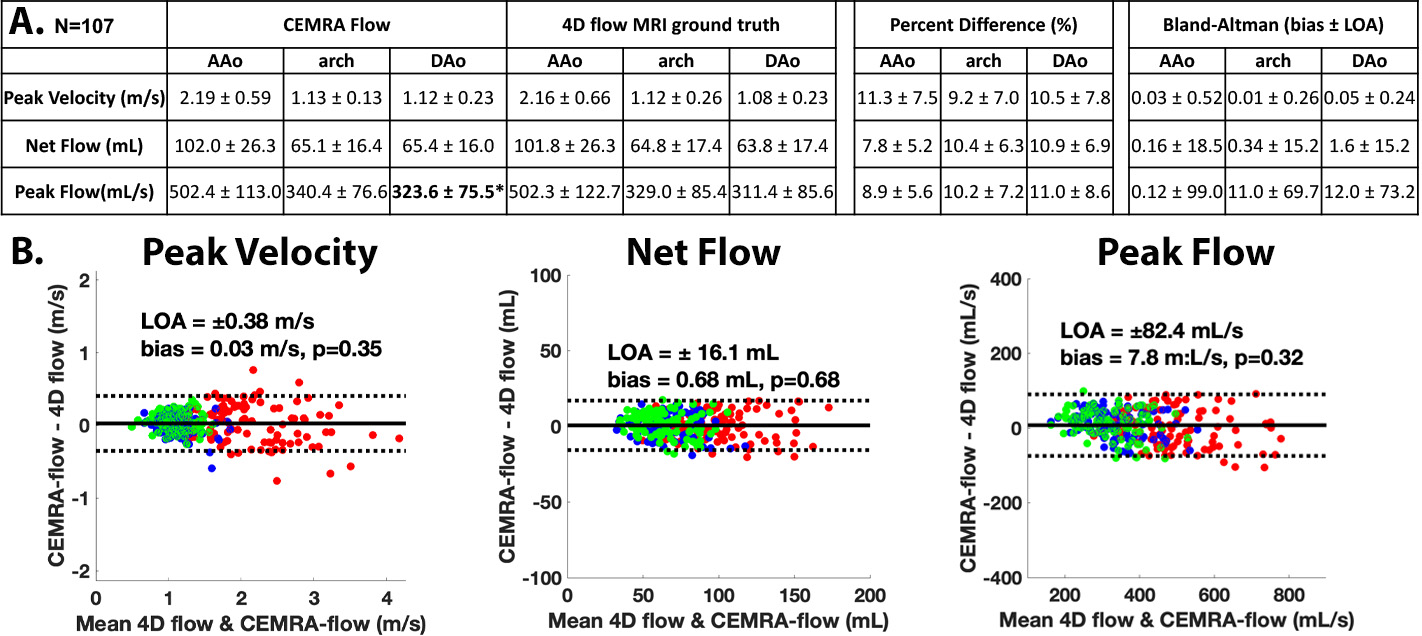
Figure 1 and 2 show examples of the AI-derived CEMRA time-resolved 3D flow in comparison to 4D flow ground-truth. Systolic and diastolic 3D velocity vector fields (Figure 1, Figure 2A) show that deep learning was able to reproduce velocities across the cardiac cycle. Figure 2B and 2C highlight excellent agreement in peak velocities and time-resolved flow. Figure 3 provides a summary of the results of Bland-Altman comparisons of regional peak velocities, net flow, and peak flow across the entire testing cohort. Low bias and strong limits of agreement were observed across all comparisons, with percent differences of 7.8-11.3% between AI derived and 4D flow ground truth data. Only peak flow in the DAo showed significant difference for AI vs. 4D flow MRI.

Conclusion:

Time-resolved AI-derived CEMRA flow showed strong agreement to the 4D flow MRI and could expand the availability of aorta hemodynamic assessment. Work is ongoing to expand this to CT angiography.

Figure 1: Outline of the deep learning pipeline to derive CEMRA flow. The testing data was the CEMRA-derived systolic velocity vector fields based on our prior work, while the input for training for the aortic geometry-derived systolic velocity vector fields. Combined with the systolic velocity input was a normalized mean velocity time curve which was calculated by grouping the datasets based on heart rates: <60 bpm, 60-69 bpm, 70-79 bpm, 80-89 bpm, 90-99 bpm, 100-109 bpm, 110-120 bpm, >120 bpm. The normalized mean velocity time curve helps to structure the input systolic velocity vector fields across time and dictates the number of timeframes for the final time-resolved output. The datasets from each group were averaged together to calculate the normalized mean velocity time cures. The inputs were fed into the 1st CNN which derives the velocity vector fields across all timeframes for each slice and then the 2nd CNN which derived the velocity vector fields across the slices for each timeframe. An example of the final output is provided showing excellent agreement to the 4D flow MRI ground-truth in systolic and diastolic velocity vector fields and time-resolved flow. S: slice, H: height, W: width, T: time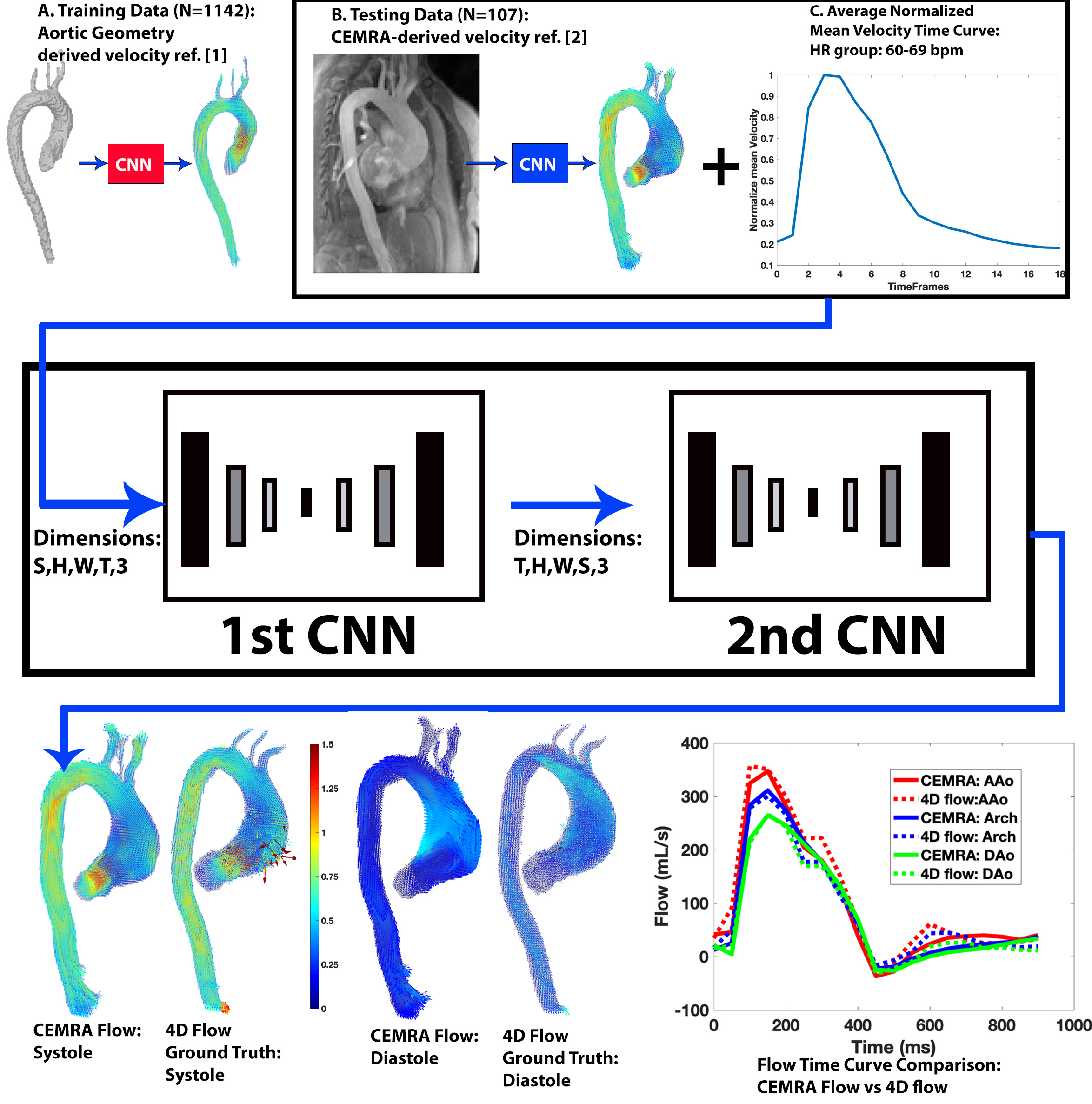

Figure 2: A: Examples of the CEMRA flow systolic and diastolic 3D velocity vector fields B: systolic velocity maximum intensity plots (MIPs). C. Plane placement and flow time curves for the CEMRA flow and 4D flow MRI ground-truth.

Figure 3: A: Table of average, regional peak velocities, net flow, and peak flow. Bland-Altman comparisons and percent difference. B: Bland-Altman plots for peak velocity, net flow, and peak flow across all datasets. Bold* indicate significant difference. LOA: limits of agreement